Learning SDR

Harvey Mudd College
Lesson 8b — Pluto Doppler RADAR
When a radio wave bounces off a moving target, its frequency shifts. This shift is called the Doppler effect. The faster the target moves, the greater the frequency shift. Our goal in this project is to build a flow diagram in GNU Radio that will transmit a pure tone in the audible range, and then receive the shifted waves that have bounced from a hand or other object that is moved towards or away from the antenna.
For speeds that are small compared to the speed of light \(c\), the frequency of a wave that reflects from a surface moving at speed \(v\) toward the transmitter is \begin{equation} f_{\rm RX} = f_{\rm TX} \times \left(1+2\frac{v}{c} \right) \end{equation} The frequency shift for a 3.5 GHz carrier wave for a speed of 3 m/s would be \begin{equation} \Delta f = 2\frac{3~\mathrm{m/s}}{3 \times 10^8~\mathrm{m/s}} (3.5 \times 10^9~\mathrm{Hz}) = 70~\mathrm{Hz} \end{equation} so we ought to be able to hear this shift, provided that we can block out the much stronger unshifted signal that goes straight from the transmit antenna to the receive antenna. We’ll use a narrow-band reject filter to do that. Finally, we will convert the complex output to a real signal that we can send to an audio sink, which will allow us to hear the shifted tone.
Equipment
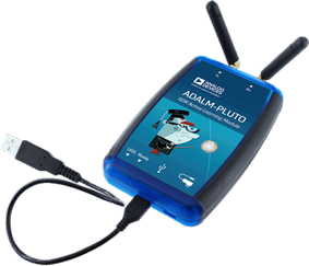
- Analog devices ADALM-PLUTO software-defined radio
Directions
-
Audio cards typically have a maximum sampling rate of 48 kHz. We will design the SDR to sample at a multiple of this frequency, so that we can down-sample the output of the radio to produce an output at 48 kHz. Set the
samp_rateto 2.4 MS/s so that when you decimate by a factor of 50 after filtering, you get 48 kHz. -
Set up four QT GUI Ranges:
tone_freq,tx_gain,rx_gain, andaudio_gain. Defaults and ranges are shown in the tables below. -
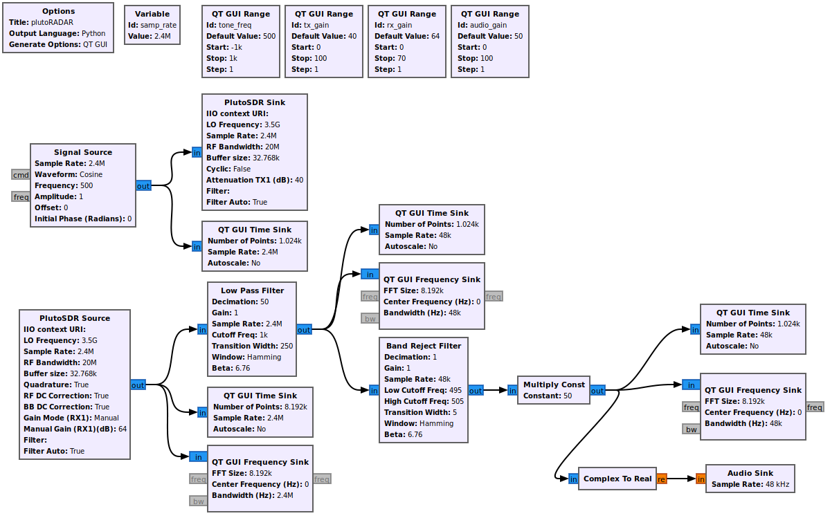
Set up a Signal Source to generate a cosine at
tone_freq. Remember that when the source is set to generate a complex output, the cosine really means \(e^{i \, 2\pi f t}\). Connect it to a PlutoSDR Sink and also display the output with a QT GUI Time Sink. You’ll need to configure the PlutoSDR to use the right local oscillator frequency and link to thetx_gainslider. Make sure to label the traces in the time sink, since you will have many plots. -
Add a PlutoSDR Source to receive the signal, display the output in the usual way (don’t forget the labels), and also send the output to a Low Pass Filter (LPF), which will roll off frequencies above 1 kHz and reduce the sample rate to the desired 48 kHz. Display the output of the LPF in the usual with (labeled) time and frequency sinks. You may find it helpful to increase the number of points used in the frequency sink by a modest power of 2 to increase the resolution.
-
Run your flow diagram and find a value of Tx attenuation that produces an undistorted sine wave on the RX plot. Note the value, so you can update the corresponding range slider’s default. Then look at the LPF frequency plot as you move your hand towards or away from the Pluto. When your hand isn’t moving, you should see the strong peak at
tone_freq, but when you move your hand, you might notice distortions in that peak, corresponding to frequencies immediately above or belowtone_freq. -
Before sending the output of the LPF to an Audio Sink, we need to strip out the strong peak at
tone_freq. Set up a Band Reject Filter (BRF), and then use a Multiply Constant block tied toaudio_gainto boost the weak signal that comes from the reflected wave. As usual, send the output also to time and frequency sinks, so you can see how effectively the band reject filter removes the strong unshifted signal at the Tx frequency. -
To hear the Doppler shifted signal, you’ll need to send the output of the BRF after it gets multiplied by the audio gain into an Audio Sink. There is a small problem: the audio sink doesn’t understand a complex signal, so we need to convert the signal using a Complex to Real block before sending it into the Audio Sink. You’ll need to set the sample rate of the audio sink to match the 48 kHz of the input signal.
Parameters
| Parameter | Value or Range |
|---|---|
| sample rate | 2.4 MS/s |
| tone frequency range | -1 kHz to 1 kHz, default 500 |
| RX gain | 0 to 70, default 64 |
| RX gain mode | manual |
| Pluto LO frequency | 3.5 GHz |
| TX attenuation | 0 to 100, default TBD |
| audio gain | 0 to 100, default 50 |
Filter properties
| Parameter | Value or Range |
|---|---|
| LPF decimation | 50 |
| LPF cutoff frequency | 2 * tone |
| LPF transition width | 250 Hz |
| LPF window | Hamming |
| BRF low cutoff frequency | tone - 5 Hz |
| BRF high cutoff frequency | tone + 5 Hz |
| BRF transition width | 5 Hz |
| BRF window | Hamming |
Things to Explore
Note: Depending on your hardware, you may find that displaying all the plots causes errors. You may find that disabling ones that arise earlier in the chain that you are not observing frees up enough computing power to avoid the errors.
-
Can you hear the chirped sound from your computer’s sound card when you move your hand rapidly towards or away from the PlutoSDR? What you hear probably lags behind the motion of your hand, since the PlutoSDR needs to send a lot of data over the USB to the computer for processing and filtering before it can be sent to the audio card.
-
In principle, you should be able to hear the shift over a range of tone frequencies. Play around a bit and figure out what frequency produces the best audio signal.
-
How does the LPF cutoff frequency affect the performance of your radio? Do you get a clearer signal with a smaller transition width on the BRF?
-
Is it easier to hear the Doppler shifted frequencies, or see them in the frequency output of the BRF?